Only released in EOL distros:
Package Summary
Adaptive Monte Carlo Localization (AMCL) in 3D.
amcl3d is a probabilistic algorithm to localizate a robot moving in 3D. It uses Monte-Carlo Localization, i.e. a particle filter. This package use a laser sensor and radio-range sensors to localizate a UAV within a known map.
- Maintainer status: maintained
- Maintainer: Francisco Cuesta Rodriguez <fcuesta AT catec DOT aero>, Paloma Carrasco Fernandez <pcarrasco AT catec DOT aero>
- Author: Francisco J.Perez-Grau <fjperez AT catec DOT aero>
- License: Apache 2.0
- Source: git https://github.com/fada-catec/amcl3d.git (branch: master)
Contents
Overview
The Adaptive Monte-Carlo Localization in 3D is a particle filter that allows you to estimate where a robot is within a 3D environment without using GPS, for example in indoor environments. This package extends previous Monte-Carlo Localization solutions meant for ground robots only, making possible to use it also with aerial robots.
The algorithm uses radio-range sensors, laser sensors, and a known map of the environment for calculating the particles weights. The algorithm takes as inputs an odometry, point-clouds that the robot sees and the distances between range sensors that are in the environment. It compares the map point-cloud with the robot point-clouds and takes into account the radio-range measurements to calculate the probability that the robot is in a bounded environment. In such environment, the particles have different weights according to each computed probability. The weighted average of all the particles would give the result of the robot pose (position and orientation).
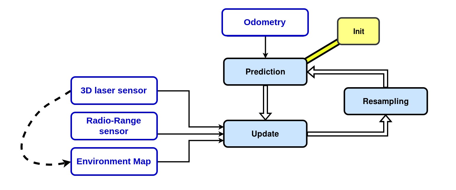
The generic Monte-Carlo algorithm has three steps: prediction, update, and resampling. This package offers one additional previous step: init. It makes it possible to initialize the robot in a given pose to start to run the algorithm. Even though this filter is able to solve the kidnapped robot problem, we propose this initialization step in order to be able to perform autonomous navigation from the very beginning of the filter execution (otherwise the estimated pose would jump until it converges to the actual pose, making the robot uncontrollable).
Prediction
Input: Odometry
Description: It is the part in charge of carrying out the propagation of the particles so that, using the input odometry, it proposes a new set of particles that potentially contain the position of the robot.
Update
Input: Map (known map of the environment), Radio-Range Sensor Measurements, 3D Laser Sensor Measurements
Description: It is responsible for evaluating the weights of the particles. It tries to verify how correctly is the pose ofeach particle by using the point-cloud of the 3D laser sensor and the measurements of the radio-range sensors. Depending on how likely each particle would receive such sensor readings at its current pose, they are assigned a corresponding weight by combining the weights computed from the two sensor technologies (laser and radio).
Resampling
Description: It is responsible for suppressing those particles that have smaller weights. Without this part, the algorithm would not converge to the correct position.
Original Paper
More information about the algorithm can be found in the following paper:
Francisco J.Perez-Grau, Fernando Caballero, Antidio Viguria and Anibal Ollero:
Multi-sensor 3D Monte Carlo Localization (MCL) for long-term aerial robot navigation, 2017
If you use amcl3d in an academic context, please cite this publication:
@article{doi:10.1177/1729881417732757,
author = {Francisco J Perez-Grau and Fernando Caballero and Antidio Viguria and Anibal Ollero},
title ={Multi-sensor three-dimensional Monte Carlo localization for long-term aerial robot navigation},
journal = {International Journal of Advanced Robotic Systems},
volume = {14},
number = {5},
year = {2017},
doi = {10.1177/1729881417732757},
URL = {https://doi.org/10.1177/1729881417732757}
}
Package files
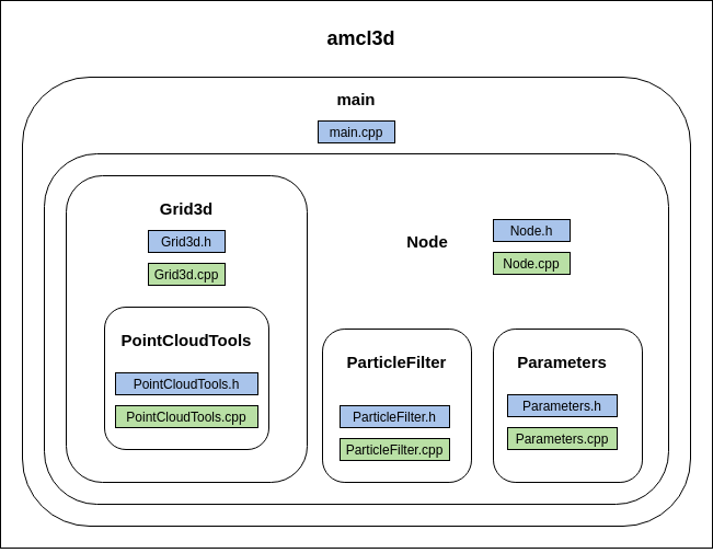
The package is structured as follows:

Source file
- [amcl3d/src]
Grid.h: defines the class "Grid3d". It works with the grid from the map.bt, opening it, building the grid message and pointcloud map and calculating compute the weights.
Grid.cpp: implements the functions of the class "!Grid3d".
PointCloudTools.h: defines the class "Grid3dCell", "Grid3dInfo" and "PointCloudInfo". It creates the grid from the map.bt, computing the weights of the grid.
PointCloudTools.cpp: implements the functions mentionated in "PointCloudTools.h". It is relationated with the information of the grid.
main.cpp: inits the function "spin" of the class "Node".
Node.cpp: implements the functions of the class "Node". It contains all the subscribers and publishers of the package, so it has the responsibility to start the map grid and follow the steps of the particle filter.
Node.h: defines the class "Node". It runs the grid and the particle filter with the parameters that were introduced into the roslaunch file.
Parameters.cpp: implements the parameter readings, and shows errors if the parameters have not been initialized, in addition to displaying the value of all of them on the screen. For more information, see section 3.1.3. Parameters.
Parameters.h: defines the class "Parameters". It declares all the generic parameters of the node.
ParticleFilter.cpp: implements the functions of the class "ParticleFilter". It has the steps mentioned before: functions of prediction, update, and resampling. Furthermore, it has other functions such as one that allows calculating the weight of the particle taking into account the error in the range sensors.
ParticleFilter.h: defines the class "ParticleFilter". It runs the steps of the Monte-Carlo method.
RViz
- [amcl3d/rviz]
amcl3d.rviz: it contains a configuration of RViz that allows displaying the topics of interest: the different point-clouds used in the algorithm, the particles, the transformations, and the localization of range-sensor.
Launch
- [amcl3d/launch]
amcl3d_rosin.launch: starts amcl3d node with a selected configuration of parameters.
roslaunch amcl3d amcl3d_rosin.launch
Msg
- [rosinrange_msg/msg]
range_pose.msg: It is the message used for the radio-range sensor measurements in the package.
For more information, see 3.2.1 Radio-Range Message.
Node
Amcl3d
The first thing the algorithm does is wait for odometry messages. If it receives them, then it waits for the robot take-off marked on the takeOffHeight_ parameter. Then, the filter begins to perform the prediction/update/resampling steps according to the point-clouds of the laser sensor and the radio-range sensor measurements, calculating particle weights. It also updates a TF for the robot.Subscribed Topics
laser_sensor (sensor_msgs/PointCloud2)- Input point-clouds from the onboard laser sensor.
- Input robot odometry.
- Input radio-range sensor measurements.
Published Topics
base_transform (geometry_msgs/TransformStamped)- It is the estimated robot TF, the result of the algorithm.
- It is the known map of the environment.
- It is the particle set.
- It is a filtered representation of the point-cloud from the robot's view (PassThrough filter in Z axis).
- It is a filtered representation of the point cloud from the robot's view (VoxelGrid filter).
- It is a graphical representation to link the radio-range sensors installed in the environment with the onboard radio-range sensor, just to check if it is receiving data from each installed sensor (it does not show the actual distance measurements).
Parameters
~base_frame_id (string)
- To set the name of the robot TF (e.g. base_link).
- To set the name of the flight origin of the robot TF (e.g. odom).
- To set the name of the test-bed origin TF (e.g. world).
- To set the route to the localization of the environment map.
- Flag to indicate if the initial pose is manually specified.
- To set the initial position in X-axis (meters).
- To set the initial position in Y-axis (meters).
- To set the initial position in Z-axis (meters).
- To set the initial yaw orientation angle (radians).
- To set dispersion of initial particle cloud in X-axis (meters).
- To set dispersion of initial particle cloud in Y-axis (meters).
- To set dispersion of initial particle cloud in Z-axis (meters).
- To set dispersion of initial particle cloud in yaw orientation (radians).
- To set the rate for publishing the map point-cloud.
- To set the Z-axis for publishing a grid slice (for debugging purposes).
- To set the rate for publishing the grid slice.
- To set the deviation of 3D laser sensor (meters).
- To set the deviation of the range sensor (meters).
- To set the size of the voxel for the VoxelGrid filter.
- To set the number of particles in the filter.
- To set the dispersion in X-axis where the filter can predict the particles (meters).
- To set the dispersion of Y-axis where the filter can predict the particles (meters).
- To set the dispersion of Z-axis where the filter can predict the particles (meters).
- To set the dispersion of yaw angle where the filter can predict the particles (radians).
- To set resampling control.
- To set the filter updating frequency.
- To set the threshold for the update in Euclidean position.
- To set the threshold for the update in yaw angle.
- To set the threshold for robot takeoff (below such height the filter will not work).
- To set the relative importance of the weight based on the point-cloud and the weight based on the radio-range sensors: alpha_*pointcloud + (1-alpha_)*range_sensor.
Rosbag
It contains several topics:
rosinrange_msg/RangePose -> It has the measurements of radio-range sensors.
sensor_msgs/PointCloud2 -> It contain the information about the pointcloud of Ouster Lidar.
sensor_msgs/Imu -> It contain the information about the IMU of Ouster Lidar.
geometry_msgs/TransformStamped -> It contains the odometry of the UAV.
Radio-Range Messages
In this case, the demo uses three sensors. One of them was mounted onboard the aerial robot, and measured distances with respect to the other two, that were statically integrated around the flight volume. The sensors used in this demo are "swarm bee ER" from Nanotron. It should be noted that the algorithm needs the distance measurements and the position of each sensor. That is why we created this message with the following structure:
Header header

uint64 source_id
uint64 destination_id
float64 range geometry_msgs/Point position
Map
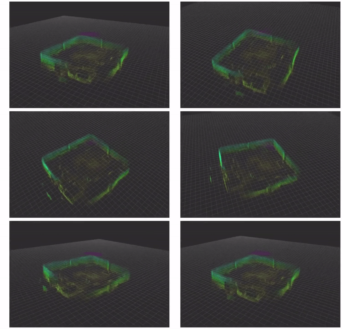
It is necessary to have a map of the environment. In this case, we have used octomap_server from Octomap to create it. Using a rosbag with VICON odometry, we have the below result:
It should be noted that the algorithm accepts both files with the extension ".bt" and ".ot". The next roslaunch itself creates the .grid from ".bt"/".ot" introduced like parameter.
roslaunch amcl3d amcl3d_rosin.launch
It probably that you have to wait several minutes to the generation of the grid.
The terminal will show you the next lines:
[ERROR] [1568280031.986394659]: [/amcl3d_node] Error opening file /home/.../mapfile_complete.grid for reading
[ INFO] [1568280031.986435846]: [/amcl3d_node] Computing 3D occupancy grid. This will take some time...
[ INFO] [1568280329.208192793]: [/amcl3d_node] Computing 3D occupancy grid done!
[ INFO] [1568280329.417065336]: [/amcl3d_node] Grid map successfully saved on /home/.../mapfile_complete.grid
TF
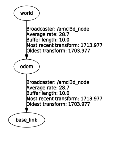
In this section, you can see the TF tree that you will find in the algorithm and the relationships among them.
world: is the origin of the map.
odom: is the odometry origin of the UAV.
base_link: is the robot frame.

Demostration Video
Acknowledgement

Supported by ROSIN - ROS-Industrial Focused Technical Projects (FTP).
More information: rosin-project.eu

