Please ask about problems and questions regarding this tutorial on answers.ros.org. Don't forget to include in your question the link to this page, the versions of your OS & ROS, and also add appropriate tags.

Splines

CubicSpline

The CubicSpline class has a relatively simple c++ interface.

• Generation of splines via blueprint algorithms.
• Access for any x, the spline value, its derivative or its second derivative.
• A streamed (algebraic) representation.

BluePrints

The blueprints generate a cubic spline over a data set. Depending on the input constraints, the spline is generated rather differently. These can be accessed via static methods in the blueprint factory (ecl::BluePrintFactory< CubicSpline >) inherited by the CubicSpline class. For example:

   1 CubicSpline cubic;
   2 cubic = CubicSpline::Natural(x_set, y_set);
   3 cubic = CubicSpline::ContinuousDerivatives(x_set, y_set, ydot_0, ydot_f);
   4 cubic = CubicSpline::DerivativeHeuristic(x_set, y_set, ydot_0, ydot_f);

Access

Access allows you to calculate the value of the spline at any point on its domain:

   1 std::cout << "Value         : " << cubic(3.2) << std::endl;
   2 std::cout << "1st Derivative: " << cubic.derivative(3.2) << std::endl;
   3 std::cout << "2nd Derivative: " << cubic.dderivative(3.2) << std::endl;

Print Algebraic Form

• Streaming will provide an algebraic list of the cubic polynomials constituting the spline.

   1 std::cout << cubic << std::endl;
   2 // Typical output
   3 // 1.00 + 2.31x + 3.00x^2 + 1.23x^3
   4 // 0.00 + 1.42x + 5.20x^2 + 1.06x^3
   5 

Smooth Linear Spline

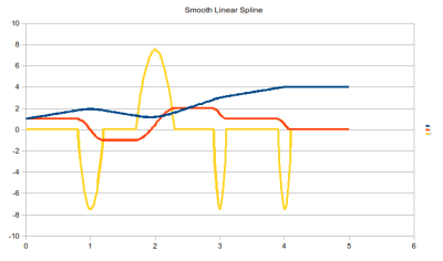
The SmoothLinearSpline simply linearly connects waypoints and adds a quintic polynomial curve to smooth the corners between each linear section. The shape of these corners is parameterised by a maximum curvature (acceleration) parameter.

Construction

Simply pass suitable x and y data sets along with a maximum curvature constraint parameter to the spline's constructor. Be sure to catch an exception if the construction should fail (this will occur if the maximum curvature constraint cannot be met).

   1 double max_curvature = 5.0;
   2 SmoothLinearSpline spline(x_set, y_set, max_curvature);

Access and streaming is similar to that for the cubic spline.

Tension Splines

A tension function is a hyperbolic function often used in spline interpolations that parameterises the tension of an interpolation between points.

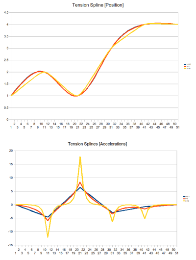
• Low tension : behaves exactly like the cubic spline
• High tension : behaves like a spline composed of piecewise smooth linear segments

The TensionSpline class is composed of a set of C2 connected tension functions.

BluePrints

There is currently only one blueprint (though variations are not difficult to create). It is very similar to the natural cubic spline (zero value boundary conditions for the second derivatives), the only difference being the addition of the tension parameter.

   1 TensionSpline spline = TensionSpline::Natural(tension, x_set, y_set);

Access and streaming is similar to that for the cubic spline.

Illustrations

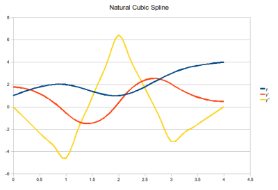
There are different ways to formulate cubic splines - the following is a natural cubic spline - it assumes zero values for the acceleration at the boundary points.

The smooth linear spline is composed of linear segments with quintics connecting them - these quintics operate at the specified maximum acceleration (curvature).

The graphs show tension splines on the same set of waypoints, but for different tension parameters. At high tension it is like a set of linear segments (with high accelerations at the joints) and at low tension, like a cubic.